Abstract
The Long Life Family Study is a genetics/genomics study of families who are identified by health records as long-lived. The study tracks family members over three generations in a series of three visits each. Each individual’s genome is fully assembled to generate genotype data, and the result of each of the three visits are measurements of a large number of phenotypes. One such phenotype measurement is whole blood RNA sequencing. Unfortunately, a mishap has occurred in at least 15 of the RNA sequence samples. These samples display a gene expression pattern which contrasts with the sex of the study subject to which the sample is attributed. To attempt to resolve this, I hypothesize that there exists a set of SNPs which are located in highly and consistently expressed exons. For each individual genome, the genotype at each SNP locus will form a vector which, like a finger print, will uniquely identify individual genomes. I can then extract the consensus base, or bases in the case of heterozygous loci, from RNA sequence library alignments and quantify the hamming distance between the RNA sequence library genotype vector and all of the individual genome genotype vectors. The result will be a ranked list which may be used to correct the mislabeled samples in the study metadata. The purpose of this project is to determine the feasibility of matching RNA sequencing libraries to individual genomes.
Introduction
This report has 5 sections, and the references, which are listed in the table of contents above. Additionally, by navigating via the top navbar on this webpage to the “Rerences” page, you may view the function definitions and source code used to generate this report and the underlying data. There are other “Articles” which detail the code used to submit scripts, which are made up of functions in this package, to a cluster scheduler. Generating this data would not have been possible on a single computer. Finally, this package will install on any computer which has an up-to-date R version installed.
Method
The genomes are assembled and genotyped in reference to human genome version hg38. A variant call file (VCF) exists for each genome which details all variants for each individual. Only high confidence single nucleotide polymorphisms over exonic regions are used for this project.
The RNA sequence reads are aligned with STAR, a splice aware aligner, to the same reference genome. Samtools pileup was used to determine the aligned base and depth over the exome for each RNA sequence library. Only reads which have a high alignment score and a depth of at least 5 are used in this project.
There are 3,688 genes which are expressed at at least 10 log2 counts per million in all of the roundly 1000 samples which have been RNA sequenced thus far. Using these regions, which are distributed over all autosomal chromosomes, I created four genotype vectors (samples of SNP loci, in other words) of length 1,900 each. Note that the number of SNPs in the SNP vector is not 1,900 – this is described in the “Nitty Gritty” details section.
As proof of concept, I selected 12 individuals with mislabeled samples. 8 of these 12 individuals have had both their visit 1 and visit 2 samples sequenced. If the sample is correctly identified to a given genome using the method I have outlined above, visit 1 and visit 2 should agree as to which genome that is. I then selected visit 1 and visit 2, where they exist, libraries for 12 other RNA sequencing samples to act as a control. These libraries pass all quality thresholds (all of the mislabels also pass these thresholds), and are not known mislabels. Since not all of the samples have both visits, there is a total of 41 RNA sequence libraries in this project, which will be compared against 4,556 individual genomes.
Literature Review
This paper describes a method of reconstructing a family pedigree from RNA sequence data. This has nearly no novel methods – they align the RNA seq reads, do some filtering, which I will address shortly, make VCF files from the output with Samtools pileup, also addressed shortly, and then use Plink, an established whole genome association software package, to create an identity by descent (IBD) matrix. The authors use the IBD matrix from Plink to infer the pedigree.
Filtering the RNA sequence reads to generate the pileup is an important step. The authors suggest stringent filters on the RNA sequence libraries. These filters are similar to those used for estimating gene expression (packages like HTSeq or Salmon). However, in applying these filters, I discovered that they are unnecessarily stringent, and thus reduce the number of bases from which we may infer the sample’s genotype.
For instance, for counting reads over a gene, it is reasonable in gene quantification applications to remove reads which multi-map with equal confidence. However, for this purpose, if the read aligns perfectly to two or more positions, it should be used at both positions to add counts to a given base. We aren’t comparing how many counts a given base has in this application – we just need to know about what base occurs at a given position in a given sample. Well aligned multi-maps do tell us that.
Similarly, the bioinformatics community has largely decided (at least in the RNA seq world) that you should not remove inferred duplicates as it is too hard to tell what is a PCR duplicate and what is a biological duplicate. Like multi-maps, if these possible duplicates align well, we should use that information.
Finally, and there are more details on this in the ‘nitty gritty’ section below, setting a mapping quality threshold (MAPQ) causes the multimaps to be removed, since the MAPQ score is reduced if a read maps to multiple locations.
In summary, this paper suggests a reasonable workflow for inferring pedigree from RNA sequence libraries. But, their suggested filters are incorrect for my application. I would argue that the filters are incorrect for their application, also, but that is not in the scope of this assignment.
This paper describes a program which the authors call BAM-matcher. This is the closest published work which I could find which describes a solution to a problem similar to the one I outline in the Introduction. The authors describe a very similar method to mine, but they match alignment files (BAMs) to other alignment files, as opposed to extracting data from Variant Call Files (VCF), and matching that data against RNAseq BAM files. I wish to use VCF files, since they a) exist and b) possess quality metrics on each SNP site already.
Furthermore, consider the VCF files as the result of thousands of BAM files. As a result, using BAM-matcher on a problem of this scale would take quite some time, and would not easily allow for exploratory data analysis.
This paper is a significant improvement on my method, though, as in the supplement it does detail the probability/statistics of matching a certain genotype at a certain site.
Method Comparison
I was not able to complete a head-on comparison for either of these methods. The data demands are far beyond that of a single local computer and I didn’t feel comfortable taking more than a day of cluster time with the amount of resources it would demand to do a reasonable comparison.
My method, on the other hand, takes a total of 2 hours to process (on a cluster) the genome VCF and RNA seq BAMs into SQLite databases. I then index the tables, which allows me to very quickly extract data and do experiments. The all-by-all hamming distance comparison is time consuming, but it can be done in parallel. On a laptop with 12 threads, it takes about an hour.
In terms of the ability to do exploratory data analysis (some of which is detailed below), this method is superior to the published methods. Of course, I have not thoroughly justified the statistics like the authors have in the BAM-Matcher paper. But, my method offers better scaling, it is extensible, and the ability to do EDA is very nice.
Nitty Gritty
Data Preparation
While it may seem trivial to extract this data, for me, at least, it was not. The genome data exists in 238 VCF files – each chromosome is split into multiple chunks – which average 4GB each. Using these files direct by reading them into memory and extracting a subset of the data, time-wise, is not not feasible. Nor is it logistically simple since each chromosome is split into at least 7 parts. As a result, it was not immediately clear how to extract and store the data to make experimentation possible.
I initially tried to use Plink, which seems to be commonly used among the geneticists at Wash U. However, for my purposes, this did not provide the quick access to the data that I needed. Simply extracting a SNP matrix (dimensions SNPs by samples) ran for more than a day without completing, and the output format (I experimented on a subset to see what it would look like) was not useful (just a huge plain text tsv).
The solution I finally arrived at was to extract the data from the VCF files into a SQLite database. Using VariantAnnotation, an R package. Using this, I could fine tune, for speed, how the data streams into my parsing program. I could also pre-filter the data so that only high quality SNPs are stored.
The table which stores the genome genotype data is called sample_genotype, and has the following fields: sample, chr (chromosome), bp (snp location, 1 indexed from the start to the end of the chromosome), ref_alt (reference genome genotype, and the alternate allele genotype, at that location, eg A/T), and genotype (three levels, A/A which represents homozygous reference, A/B which represents a heterzygous locus, and B/B for homozygous alternate). This table is indexed on sample, chr and bp for fast lookup.
One useful feature of using a database framework is that I can also create views, or virtual tables defined by a SQL query of other tables in the database, which define the randomly sampled sets of loci to be used to match genomes to RNA sequence libraries. For example, the SQL command which creates the first sample looks like this:
DROP VIEW IF EXISTS "main"."sample1";
CREATE VIEW "sample1" AS
SELECT * FROM sample_genotype
WHERE (chr IS 13.0 AND bp BETWEEN 48975912 AND 49209779 OR
       ...
       chr IS 17.0 AND bp BETWEEN 50962174 AND 51120868 OR
       ...
       chr IS 19.0 AND bp BETWEEN 12995475 AND 13098796 OR
       ...
For each RNA sequence library, I used Rsamtools, an R wrapper for Samtools, to ‘pileup’ the alignments from the BAM files. There are more details on the filters which I used in the section below.
Sample Preparation
The genome SNP variants are sampled from 4000 highly and consistently expressed gene ranges. To reduce the time for each distance calculation, rather than using all 4000 regions to extract SNP vectors, I created 4 samples of 1,900 gene ranges drawn from the 4,000 genes. I then intersected those samples with the genome SNP database. The result of this is a list of SNPS which occur in the sampled regions in the individual genomes. For sample1, for example, there are 840 high confidence SNPS.
> snp_df
# A tibble: 840 × 2
   chr         bp
   <chr>    <int>
 1 12.0  12500010
 2 12.0  12500075
 3 12.0  12500375
 4 12.0  12500383
 5 12.0  12500396
 6 12.0  12500480
 7 12.0  12500556
 8 12.0  12500807
 9 12.0  12500824
10 12.0  12500914
# … with 830 more rows
Using this, I then create a SNP vector for each of the 4,556 individual genomes. A subset of one SNP vector looks like this, where ‘8’ is the subject ID:
> sample_genome_vectors$`8`
  [1] "G"         "G"         "G"         "C"         "G"
  [6] "G"         "A"         "G"         "C"         "G"
 [11] "G"         "G"         "T"         "G"         "A"
 [16] "T"         "A"         "G"         "A"         "A"
 [21] "A"         "T"         "A"         "G"         "G"
 [26] "A"         "C"         "C"         "T"         "A"
 [31] "T"         "T"         "C"         "T"         "C"
 [36] "C"         "T"         "T"         "C"         "G"
 [41] "C"         "C"         "A"         "G"         "T"
 ...
Using the exact base pair coordinates of these SNPs, I then extract the consensus base at the same location from each of the RNA sequence libraries. For any location which does not have enough depth due to coverage or quality filters, the value “Uncertain” is entered:
> pileup_vector
  [1] "G"         "G"         "G"         "C"         "G"
  [6] "G"         "A"         "G"         "C"         "G"
 [11] "G"         "Uncertain" "Uncertain" "Uncertain" "Uncertain"
 [16] "Uncertain" "Uncertain" "Uncertain" "Uncertain" "Uncertain"
 [21] "Uncertain" "Uncertain" "Uncertain" "Uncertain" "Uncertain"
 [26] "A"         "Uncertain" "Uncertain" "Uncertain" "Uncertain"
 [31] "Uncertain" "T"         "Uncertain" "Uncertain" "C"
 [36] "C"         "Uncertain" "Uncertain" "Uncertain" "Uncertain"
 [41] "C"         "Uncertain" "Uncertain" "Uncertain" "Uncertain"
 ...
After generating this data, I was concerned at how many “Uncertain” positions there are, especially over highly expressed genes. Thus, I explored the alignments themselves:
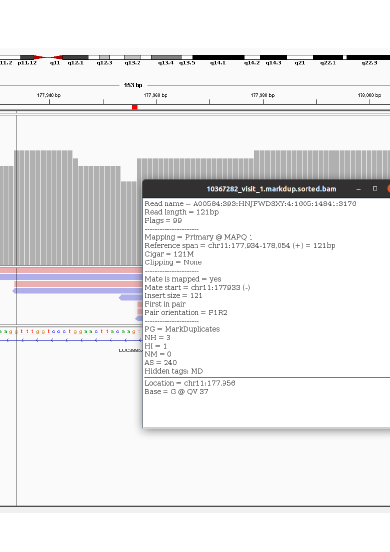
Figure 1: An RNAseq library SNP locations
The vertical bar in figure 1 is over the first “Uncertain” locus in the alignment from which the pileup vector above originates. The detail box in the image gives details on one of the reads which overlaps this base. It says the following: The read is 121 base pairs long. SAM flag 99 means that this read, along with its pair, are both mapped (the library is unstranded, so in this case, R1 maps to the forward strand while R2 maps to the reverse strand). This location is the primary alignment for this read, and it aligns without gaps (Cigar 121M means 121 matches). Furthermore, the tag AS is the “alignment score” (note that alignment score is the score of the actual smith waterman type alignment while MAPQ is a ‘mapping score’ which takes into account multi-mapping) and it 240 out of a possible 244. There is no soft clipping at the ends of the read and the mate is also mapped.
However, the mapping quality (MAPQ) is 1. That indicates that this alignment may occur with ~70% chance in other locations in the genome. And, this is the case: the flag NH:3 means that there are 3 other alignments which are as good as this one. Note that a ‘supplemental alignment’ is an alignment which has a lesser score than the primary alignment. This is different than a ‘secondary alignment’ which is an alignment as good as the primary alignment. The location called primary is arbitrary if a read multi-maps with secondary alignments.
In thinking about this, I realized that the more stringent MAPQ filter on the pileup step, while reasonable for something like RNA sequencing, is not necessary for this purpose. A high quality multi-map does provide evidence of a given base’s identity. In fact, it increases confidence. Thus, I decided to re-do the pileup and to only set base_quality score. Furthermore, I decided to count both primary and secondary alignments. This marks a significant departure from the ‘Inferring identity …’ paper.
The result is fewer ‘Uncertain’ base locations in the RNA sequence library pileups (Figure 1).
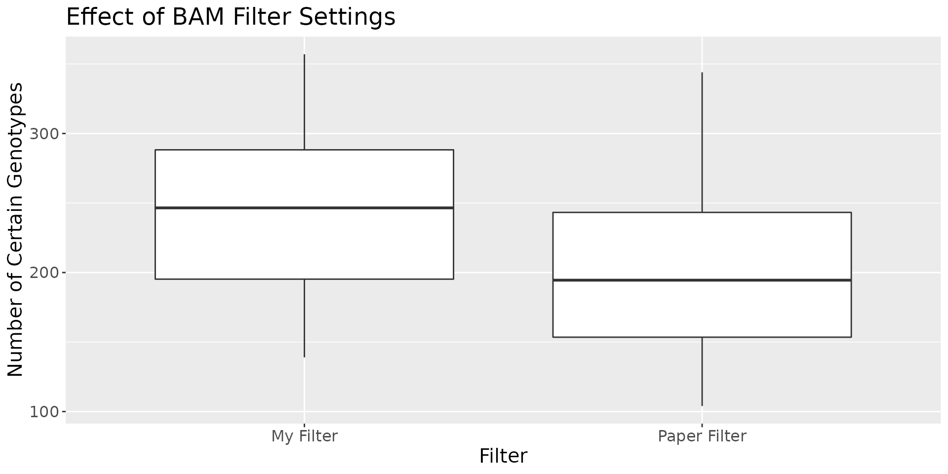
Figure 1: Comparing the number of uncertain bases with different filters
Figure 1 shows the distribution of “Certain Genotypes”, by which I mean genotypes which have adequate coverage and alignment quality in the RNA seq, which are identified as SNPs in the VCFs, and which are in highly and consistently expressed gene regions. Using my filters, which count bases in reads in all good alignments, regardless of whether or not the read is identified as a multimap, significantly increases the number of “certain genotypes”. The average length, using these new filters, in any given SNP vector in any given sample, is slightly less than 250. This is the effective length of any SNP vector, and it is only across these “certain genotypes” that the equivalence class based hamming distance (see below) is calculated. The denominator for the “difference ratio” (also below) is the number of ‘certain bases’ in a given SNP vector.
Distance
The ‘equivalence class based hamming distance’ between an RNA sequence library SNP vector and an individual’s genome SNP vector is calculated using one of the two scoring matrices below. The strict matrix only accepts exact matches where the homozygous bases match each other, and heterozygous match in either order, e.g. A/T == T/A.
The lenient scoring matrix, on the other hand, allows matches also among heterozygous genotypes which include the same base. For instance, A matches A/A, and any heterozygous genotype with A.
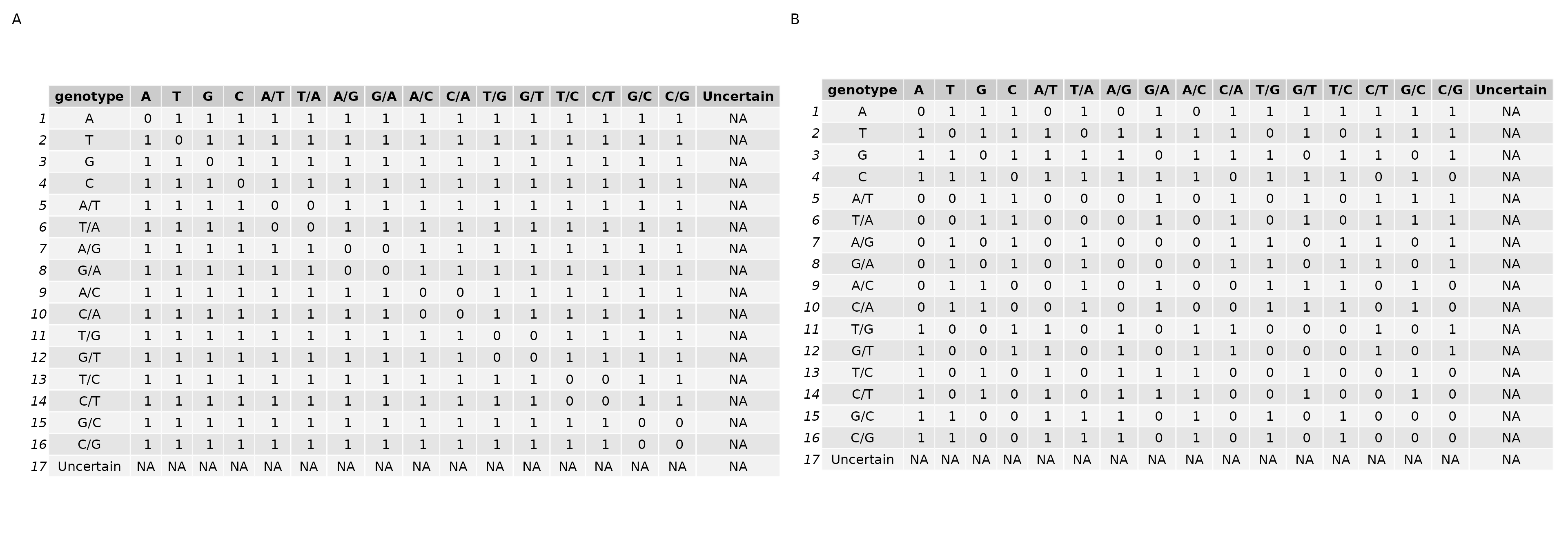
Figure 2: Strict and Lenient Scoring Matricies
I experimented with both matricies, and I ultimately chose the ‘strict’ matrix for all of the following results.
Time and Space
The raw individual genome data is about 1TB. As a SQLite database, it is reduced to 5GB. I sampled 40 RNA seq libraries. The SQLite databases which result from the ‘pileup’ are about 5GB each. Preprocessing, on a cluster, takes a total of 1 to 2 hours depending on how quickly the jobs are scheduled. Reading the data into the databases, which is O(N) in the size of the file, takes about 30 minutes for each file. Indexing the databases is included in this time.
Once the databases are created, extracting data, due to the indicies, is fast. Calculating the hamming distance is O(MNS) where M is the number of RNA seq libraries, N is the number of genomes, and S is the length of the SNP vector. The result is a square matrix where the dimensions are the number of RNAseq libraries vs the number of genomes, and the entries are the distance ratio between the SNP vectors. In this case, the number of computations are 40*4556*1000. In parallel on a laptop, this takes about an hour.
Results
In this study, there are 4 independently drawn samples of SNP genome vectors from 1,900 gene regions. The genomic SNP vectors which result are, on average, of length 840. Using these genomic SNP vectors, I then generate SNP vectors in the RNA sequence libraries. On average, these RNA seq SNP vectors have 250 ‘Certain Bases’ (see Figure 1), and these ‘Certain Bases’ are the vectors over which the equivalence class based hamming distance comparison will occur.
After generating the 4 sample genomic and RNA seq SNP vectors, I initially investigated how similar the SNP vectors are to one another by comparing genomic SNP vectors against the genomic SNP vectors, and the RNA seq SNP vectors against the RNA seq SNP vectors. What is revealed is that there are 38 individual genomes with SNP vectors in at least 1 of the 4 samples which match another individual exactly. By contrast, none of the RNA seq vectors match one another exactly.
Figure 3, below, describes the results of this experiment for both the genomic SNP vectors (Figure 3A), and the RNA seq vectors (Figure 3B). In each table, there are two columns, Metric and Value. These tables represent measurements of the number of differences between SNP vectors. The metrics represented are: Number of Exact Matches, the first percentile, median, mean, third percentile and maximum number of differences between genome SNP vectors. This is calculated using the ‘strict’ difference matrix above (Figure 2) over the 4 independently drawn samples.
Being unable to differentiate between genomes is obviously a problem. However, the remedy is likely to increase the number of regions over which I sample SNPs. As this is a proof of concept, the goal is not necessarily to unambiguously match libraries to genomes in this experiment, but to show that this method is reasonable and yields consistent results. As such, what we would expect is for the RNAseq libraries which match to one of the 38 genomes which are exactly the same to match with the same score to all genomes.
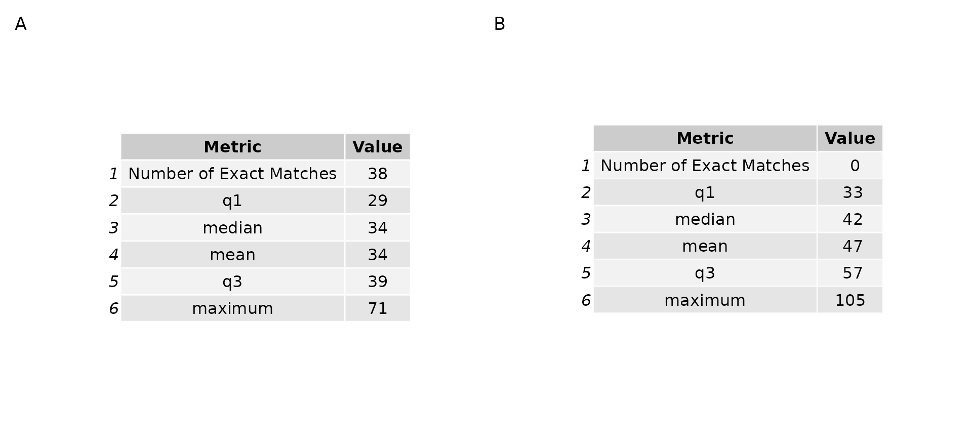
Figure 3: Comparing genome and RNAseq library pileup SNP vectors
I next compared all of the 41 RNA seq SNP vectors against all of the 4,556 genomic SNP vectors. Figure 4 below shows the results of the experiment in matching pile up SNP vectors to genome vectors of the same SNPs using the ‘strict’ scoring matrix. Figure 4A, on the left, are the samples which are expected to be correctly labelled. Figure 4B are the known mislabels. The top scoring (lowest difference ratio) “inferred” subject ID is selected for each rnaseq pileup. For instance, if RNAseq library 1 has a difference ratio of 0 to genome 3, then the ‘inferred’ label for this the RNAseq library currently labelled 1 is 3.
#> Joining, by = "subject"
#> Selecting by mean_diff_ratio
#> Selecting by mean_diff_ratio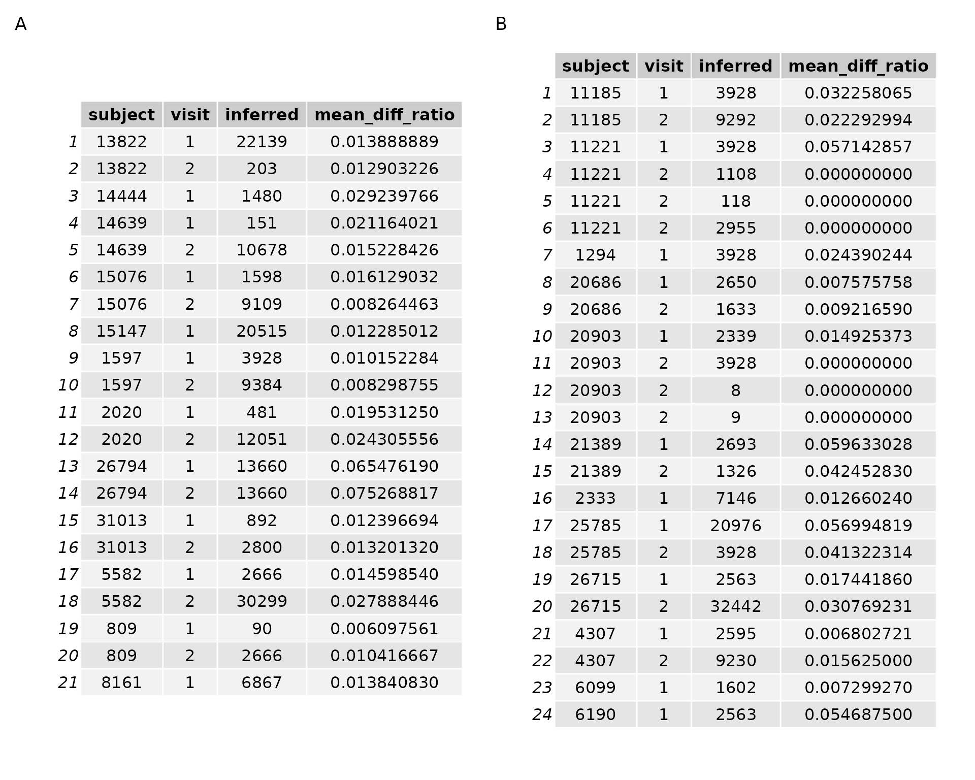
Figure 4: RNA seq vs all genomes results
What we see is that not a single subject is inferred to be the same as that which it is labelled. This is disturbing, since there are 21 samples which have been included that are expected to be correctly labelled.
I am confident in the SNP strings that I am extracting – I know I am extracting genotypes for certain samples with a given label from the sample metadata, and matching those genotypes to the corresponding RNAseq base. However, the depth over any given base in the RNAseq data is frequently very low. RNA is not as stable as DNA, so possibly there are more cases in which a base is called as heterozygous due to sequencing error. Another possibility is that there simply need to be more SNPs included, though the time to extract ‘genome length’ SNPs and do the processing is such that I hesitate to do so when this method seems to yield poor results already. Finally, it is also possible that there are a lot more mislabels than we expect or hope, though I think this is not likely. If it were the case, presumably there are still more correctly labelled samples than incorrectly labelled samples. I should, therefore, be matching subject to ID more often than chance. I could test this by increasing the number of subjects which I examine.
Conclusion
This project tested whether or not it is possible to extract from individual genomes a set of SNPs over highly and consistently expressed genes which could be used as a ‘finger print’ with which we may match the individual genome to a corresponding RNA sequence library. To test this, I created a database of genotypes for 4,556 samples. I next identified abou 3,688 highly and consistently expressed genes, and created 4 samples of around 1,900 base pair locations. With these samples, I extracted the consensus base(s) over each of the 840 base locations from 40 RNAseq libraries. The resulting “Certain Bases” in the RNA seq vectors number, on average, 250 genotypes in length. I then calculated the equivalence class based hamming distance (Figure 2) between all genome SNP vectors, all RNA seq SNP vectors, and between the genome SNP vectors and RNA sequence SNP vectors.
My finding is that my current method does not, with high confidence, match genomes to RNAseq libraries. It is possible that increasing the amount of data, either by expanding the gene set or by including more RNA seq libraries, could yield results.